HOW LSI WORKS

The Search for Content

We mentioned that latent semantic indexing looks at patterns of word distribution (specifically, word co-occurence) across a set of documents. Before we talk about the mathematical underpinnings, we should be a little more precise about what kind of words LSI looks at.

Natural language is full of redundancies, and not every word that appears in a document carries semantic meaning. In fact, the most frequently used words in English are words that don't carry content at all: functional words, conjunctions, prepositions, auxilliary verbs and others. The first step in doing LSI is culling all those extraeous words from a document, leaving only content words likely to have semantic meaning. There are many ways to define a content word - here is one recipe for generating a list of content words from a document collection:

1. Make a complete list of all the words that appear anywhere in the collection
2. Discard articles, prepositions, and conjunctions
3. Discard common verbs (know, see, do, be)
4. Discard pronouns
5. Discard common adjectives (big, late, high)
6. Discard frilly words (therefore, thus, however, albeit, etc.)
7. Discard any words that appear in every document
8. Discard any words that appear in only one document

This process condenses our documents into sets of content words that we can then use to index our collection.

Thinking Inside the Grid

Using our list of content words and documents, we can now generate a term-document matrix. This is a fancy name for a very large grid, with documents listed along the horizontal axis, and content words along the vertical axis. For each content word in our list, we go across the appropriate row and put an 'X' in the column for any document where that word appears. If the word does not appear, we leave that column blank.

Doing this for every word and document in our collection gives us a mostly empty grid with a sparse scattering of X-es. This grid displays everthing that we know about our document collection. We can list all the content words in any given document by looking for X-es in the appropriate column, or we can find all the documents containing a certain content word by looking across the appropriate row.

Notice that our arrangement is binary - a square in our grid either contains an X, or it doesn't. This big grid is the visual equivalent of a generic keyword search, which looks for exact matches between documents and keywords. If we replace blanks and X-es with zeroes and ones, we get a numerical matrix containing the same information.

The key step in LSI is decomposing this matrix using a technique called singular value decomposition. The mathematics of this transformation are beyond the scope of this article (a rigorous treatment is available here), but we can get an intuitive grasp of what SVD does by thinking of the process spatially. An analogy will help.

Breakfast in Hyperspace

Imagine that you are curious about what people typically order for breakfast down at your local diner, and you want to display this information in visual form. You decide to examine all the breakfast orders from a busy weekend day, and record how many times the words bacon, eggs and coffee occur in each order.

You can graph the results of your survey by setting up a chart with three orthogonal axes - one for each keyword. The choice of direction is arbitrary - perhaps a bacon axis in the x direction, an eggs axis in the y direction, and the all-important coffee axis in the z direction. To plot a particular breakfast order, you count the occurence of each keyword, and then take the appropriate number of steps along the axis for that word. When you are finished, you get a cloud of points in three-dimensional space, representing all of that day's breakfast orders.

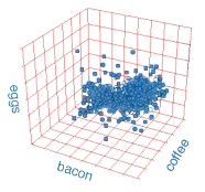
If you draw a line from the origin of the graph to each of these points, you obtain a set of vectors in 'bacon-eggs-and-coffee' space. The size and direction of each vector tells you how many of the three key items were in any particular order, and the set of all the vectors taken together tells you something about the kind of breakfast people favor on a Saturday morning.

What your graph shows is called a term space. Each breakfast order forms a vector in that space, with its direction and magnitude determined by how many times the three keywords appear in it. Each keyword corresponds to a separate spatial direction, perpendicular to all the others. Because our example uses three keywords, the resulting term space has three dimensions, making it possible for us to visualize it. It is easy to see that this space could have any number of dimensions, depending on how many keywords we chose to use. If we were to go back through the orders and also record occurences of sausage, muffin, and bagel, we would end up with a six-dimensional term space, and six-dimensional document vectors.

Applying this procedure to a real document collection, where we note each use of a content word, results in a term space with many thousands of dimensions. Each document in our collection is a vector with as many components as there are content words. Although we can't possibly visualize such a space, it is built in the exact same way as the whimsical breakfast space we just described. Documents in such a space that have many words in common will have vectors that are near to each other, while documents with few shared words will have vectors that are far apart.

Latent semantic indexing works by projecting this large, multidimensional space down into a smaller number of dimensions. In doing so, keywords that are semantically similar will get squeezed together, and will no longer be completely distinct. This blurring of boundaries is what allows LSI to go beyond straight keyword matching. To understand how it takes place, we can use another analogy.

Singular Value Decomposition

Imagine you keep tropical fish, and are proud of your prize aquarium - so proud that you want to submit a picture of it to Modern Aquaria magazine, for fame and profit. To get the best possible picture, you will want to choose a good angle from which to take the photo. You want to make sure that as many of the fish as possible are visible in your picture, without being hidden by other fish in the foreground. You also won't want the fish all bunched together in a clump, but rather shot from an angle that shows them nicely distributed in the water. Since your tank is transparent on all sides, you can take a variety of pictures from above, below, and from all around the aquarium, and select the best one.

In mathematical terms, you are looking for an optimal mapping of points in 3-space (the fish) onto a plane (the film in your camera). 'Optimal' can mean many things - in this case it means 'aesthetically pleasing'. But now imagine that your goal is to preserve the relative distance between the fish as much as possible, so that fish on opposite sides of the tank don't get superimposed in the photograph to look like they are right next to each other. Here you would be doing exactly what the SVD algorithm tries to do with a much higher-dimensional space.

Instead of mapping 3-space to 2-space, however, the SVD algorithm goes to much greater extremes. A typical term space might have tens of thousands of dimensions, and be projected down into fewer than 150. Nevertheless, the principle is exactly the same. The SVD algorithm preserves as much information as possible about the relative distances between the document vectors, while collapsing them down into a much smaller set of dimensions. In this collapse, information is lost, and content words are superimposed on one another.

Information loss sounds like a bad thing, but here it is a blessing. What we are losing is noise from our original term-document matrix, revealing similarities that were latent in the document collection. Similar things become more similar, while dissimilar things remain distinct. This reductive mapping is what gives LSI its seemingly intelligent behavior of being able to correlate semantically related terms. We are really exploiting a property of natural language, namely that words with similar meaning tend to occur together.

< previous     next >

This work is licensed under a Creative Commons License. 2002 National Institute for Technology in Liberal Education. For more info, contact the author.

Gain a Competitive Advantage Today

Your top competitors have been investing into their marketing strategy for years.

Now you can know exactly where they rank, pick off their best keywords, and track new opportunities as they emerge.

Explore the ranking profile of your competitors in Google and Bing today using SEMrush.

Enter a competing URL below to quickly gain access to their organic & paid search performance history - for free.

See where they rank & beat them!